Benchmark adsorption and surface energies with RPA

This database contains the adsorption energies of 200 reactions involving 8 different adsorbates on 25 different transition metal surfaces at full coverage as well as the surface energies for the same surfaces. Various DFT functionals have been employed and compared to the results from many-body perturbation theory within the random phase approximation.

The adsorption reactions are

1. \(\mathrm{H}_2\mathrm{O} + \mathrm{slab} \rightarrow \mathrm{OH/slab} + \frac{1}{2} \mathrm{H}_2\)

2. \(\mathrm{CH}_4 + \mathrm{slab} \rightarrow \mathrm{CH/slab} + \frac{3}{2} \mathrm{H}_2\)

3. \(\mathrm{NO} + \mathrm{slab} \rightarrow \mathrm{NO/slab}\)

4. \(\mathrm{CO} + \mathrm{slab} \rightarrow \mathrm{CO/slab}\)

5. \(\mathrm{N}_2 + \mathrm{slab} \rightarrow \mathrm{N_2/slab}\)

6. \(\frac{1}{2}\mathrm{N}_2 + \mathrm{slab} \rightarrow \mathrm{N/slab}\)

7. \(\frac{1}{2}\mathrm{O}_2 + \mathrm{slab} \rightarrow \mathrm{O/slab}\)

8. \(\frac{1}{2}\mathrm{H}_2 + \mathrm{slab} \rightarrow \mathrm{H/slab}\)

and the surfaces include 3d transition metals from Scandium (Sc) to Zink (Zn), 4d from Yttrium (Y) to Cadmium (Cd) excluding Technetium (Tc) and 5d from Hafnium (Hf) to Gold (Au).

Per S. Schmidt and Kristian S. Thygesen

Benchmark Database of Transition Metal Surface and Adsorption Energies from Many-Body Perturbation Theory

The Journal of Physical Chemistry C Article ASAP

The data can be obtained from the files:

• Download raw data adsorption.db and surfaces.db

And browsed online:

• Browse adsorption energies

• Browse surface energies

The adsorption energy is defined with respect to the adsorbate in its gas phase: \(E_{\text{ads}} = E_{\text{adsorbate@slab}} - (E_{\text{slab}} + E_{\text{adsorbate(g)}})\)

And the surface energy as: \(E_{\text{surf}} = \frac12 \bigg( E_{\text{slab}} - N_{\text{layers}} E_{\text{bulk}}\bigg)\), where the number of atomic layers in the slab is \(N_{\text{layers}} = 3\).

One example reaction that the adsorption energy is calculated for is:

\(\mathrm{CH}_4\mathrm{(g)} + \mathrm{Sc} \rightarrow \mathrm{CH/Sc} + \frac32 \mathrm{H}_2\mathrm{(g)}\)

In the database the adsorbate is then \(\mathrm{CH}\), the surface material is \(\mathrm{Sc}\), reference molecule 1 is \(\mathrm{CH}_4\) and reference molecule 2 is \(\mathrm{H}_2\). The adsorption energy is then \(E_{\text{ads}} = E_{\mathrm{CH/Sc}} -(E_{\mathrm{Sc}} + E_{\mathrm{CH}_4\mathrm{(g)}} - \frac32 E_{\mathrm{H}_2\mathrm{(g)}})\).

Key-value pairs

Database of adsorption energies:

key	description	unit
BEEFvdW_ads	BEEF-vdW adsorbate on slab	eV
BEEFvdW_adsorp	Adsorption energy with BEEF-vdW	eV
BEEFvdW_mol	BEEF-vdW 1st molecule	eV
BEEFvdW_mol2	BEEF-vdW 2nd molecule	eV
BEEFvdW_slab	BEEF-vdW slab	eV
EXX_ads	EXX adsorbate on slab	eV
EXX_adsorp	Adsorption energy with EXX	eV
EXX_mol	EXX 1st molecule	eV
EXX_mol2	EXX 2nd molecule	eV
EXX_slab	EXX slab	eV
LDA_ads	LDA adsorbate on slab	eV
LDA_adsorp	Adsorption energy with LDA	eV
LDA_mol	LDA 1st molecule	eV
LDA_mol2	LDA 2nd molecule	eV
LDA_slab	LDA slab	eV
PBE_ads	PBE adsorbate on slab	eV
PBE_adsorp	Adsorption energy with PBE	eV
PBE_mol	PBE 1st molecule	eV
PBE_mol2	PBE 2nd molecule	eV
PBE_slab	PBE slab	eV
RPA_EXX_adsorp	Adsorption energy with EXX+RPA	eV
RPA_ads_ecut300_k12	RPA adsorbate on slab, Ecut=300, k=12x12x1	eV
RPA_ads_ecut300_k6	RPA adsorbate on slab, Ecut=300, k=6x6x1	eV
RPA_ads_ecut400_k6	RPA adsorbate on slab, Ecut=400, k=6x6x1	eV
RPA_ads_ecut500_k6	RPA adsorbate on slab, Ecut=500, k=6x6x1	eV
RPA_ads_extrap	RPA adsorbate on slab extrapolated	eV
RPA_adsorp	RPA correlation adsorption energy extrapolated	eV
RPA_mol2_ecut425	RPA 2nd molecule, Ecut=425	eV
RPA_mol2_ecut450	RPA 2nd molecule, Ecut=450	eV
RPA_mol2_ecut475	RPA 2nd molecule, Ecut=475	eV
RPA_mol2_ecut500	RPA 2nd molecule, Ecut=500	eV
RPA_mol2_ecut530	RPA 2nd molecule, Ecut=530	eV
RPA_mol2_ecut560	RPA 2nd molecule, Ecut=560	eV
RPA_mol2_ecut600	RPA 2nd molecule, Ecut=600	eV
RPA_mol2_extrap	RPA 2nd molecule extrapolated	eV
RPA_mol_ecut425	RPA 1st molecule, Ecut=425	eV
RPA_mol_ecut450	RPA 1st molecule, Ecut=450	eV
RPA_mol_ecut475	RPA 1st molecule, Ecut=475	eV
RPA_mol_ecut500	RPA 1st molecule, Ecut=500	eV
RPA_mol_ecut530	RPA 1st molecule, Ecut=530	eV
RPA_mol_ecut560	RPA 1st molecule, Ecut=560	eV
RPA_mol_ecut600	RPA 1st molecule, Ecut=600	eV
RPA_mol_extrap	RPA 1st molecule extrapolated	eV
RPA_slab_ecut300_k12	RPA slab, Ecut=300, k=12x12x1	eV
RPA_slab_ecut300_k6	RPA slab, Ecut=300, k=6x6x1	eV
RPA_slab_ecut400_k6	RPA slab, Ecut=400, k=6x6x1	eV
RPA_slab_ecut500_k6	RPA slab, Ecut=500, k=6x6x1	eV
RPA_slab_extrap	RPA slab extrapolated	eV
RPBE_ads	RPBE adsorbate on slab	eV
RPBE_adsorp	Adsorption energy with RPBE	eV
RPBE_mol	RPBE 1st molecule	eV
RPBE_mol2	RPBE 2nd molecule	eV
RPBE_slab	RPBE slab	eV
adsorbate	Adsorbate
mBEEF_ads	mBEEF adsorbate on slab	eV
mBEEF_adsorp	Adsorption energy with mBEEF	eV
mBEEF_mol	mBEEF 1st molecule	eV
mBEEF_mol2	mBEEF 2nd molecule	eV
mBEEF_slab	mBEEF slab	eV
mBEEFvdW_ads	mBEEF-vdW adsorbate on slab	eV
mBEEFvdW_adsorp	Adsorption energy with mBEEF-vdW	eV
mBEEFvdW_mol	mBEEF-vdW 1st molecule	eV
mBEEFvdW_mol2	mBEEF-vdW 2nd molecule	eV
mBEEFvdW_slab	mBEEF-vdW slab	eV
mol	Reference molecule 1
mol2	Reference molecule 2
surf_mat	Surface Material
vdWDF2_ads	vdW-DF2 adsorbate on slab	eV
vdWDF2_adsorp	Adsorption energy with vdW-DF2	eV
vdWDF2_mol	vdW-DF2 1st molecule	eV
vdWDF2_mol2	vdW-DF2 2nd molecule	eV
vdWDF2_slab	vdW-DF2 slab	eV

Similar for the surface energies:

key	description	unit
BEEFvdW_bulk	BEEF-vdW bulk	eV
BEEFvdW_slab	BEEF-vdW slab	eV
BEEFvdW_surf	Surface energy with BEEF-vdW	eV
EXX_bulk	EXX bulk	eV
EXX_slab	EXX slab	eV
EXX_surf	Surface energy with EXX	eV
LDA_bulk	LDA bulk	eV
LDA_slab	LDA slab	eV
LDA_surf	Surface energy with LDA	eV
PBE_bulk	PBE bulk	eV
PBE_slab	PBE slab	eV
PBE_surf	Surface energy with PBE	eV
RPA_EXX_surf	Surface energy with EXX+RPA	eV
RPA_bulk_ecut300_k12	RPA bulk, Ecut=300, k=12x12x12	eV
RPA_bulk_ecut400_k12	RPA bulk, Ecut=400, k=12x12x12	eV
RPA_bulk_ecut500_k12	RPA bulk, Ecut=500, k=12x12x12	eV
RPA_bulk_extrap	RPA bulk extrapolated	eV
RPA_slab_ecut300_k12	RPA slab, Ecut=300, k=12x12x1	eV
RPA_slab_ecut300_k6	RPA slab, Ecut=300, k=6x6x1	eV
RPA_slab_ecut400_k6	RPA slab, Ecut=400, k=6x6x1	eV
RPA_slab_ecut500_k6	RPA slab, Ecut=500, k=6x6x1	eV
RPA_slab_extrap	RPA slab extrapolated	eV
RPA_surf	RPA correlation surface energy extrapolated	eV
RPBE_bulk	RPBE bulk	eV
RPBE_slab	RPBE slab	eV
RPBE_surf	Surface energy with RPBE	eV
mBEEF_bulk	mBEEF bulk	eV
mBEEF_slab	mBEEF slab	eV
mBEEF_surf	Surface energy with mBEEF	eV
mBEEFvdW_bulk	mBEEF-vdW bulk	eV
mBEEFvdW_slab	mBEEF-vdW slab	eV
mBEEFvdW_surf	Surface energy with mBEEF-vdW	eV
surf_mat	Material
vdWDF2_bulk	vdW-DF2 bulk	eV
vdWDF2_slab	vdW-DF2 slab	eV
vdWDF2_surf	Surface energy with vdW-DF2	eV

Reading data

In the following script it is shown how to extract and plot adsorption and surface energies from the database files (adsorption.db, surfaces.db):

# creates: database_example.svg
import numpy as np
import matplotlib.pyplot as plt
import ase.db

adsorbate = 'NO'
slabs = ['Sc', 'Ti', 'Cu', 'Pd']
db = ase.db.connect('adsorption.db')
db_surf = ase.db.connect('surfaces.db')

labels = ['LDA', 'PBE', 'RPBE', 'BEEF-vdW', 'RPA']
markers = ['o', 's', 'v', 'D', 'x']
markersize = [10, 10, 10, 10, 12]
mews = [1, 1, 1, 1, 4]
cols = ['r', 'k', 'b', 'g']

plt.figure()
for ii, slab in enumerate(slabs):
    rows = db.select(adsorbate=adsorbate)
    adss = []
    for row in rows:
        if row.symbols[0] == slab:
            adss.append(row.LDA_adsorp)
            adss.append(row.PBE_adsorp)
            adss.append(row.RPBE_adsorp)
            adss.append(row.BEEFvdW_adsorp)
            adss.append(row.RPA_EXX_adsorp)

    rows_surf = db_surf.select(surf_mat=slab)
    surfs = []
    for row in rows_surf:
        surfs.append(row.LDA_surf)
        surfs.append(row.PBE_surf)
        surfs.append(row.RPBE_surf)
        surfs.append(row.BEEFvdW_surf)
        surfs.append(row.RPA_EXX_surf)

    for i in range(len(adss)):
        if ii == 0:
            plt.plot(surfs[i], adss[i], color='darkgray',
                     marker=markers[i], markersize=markersize[i],
                     mew=mews[i], label=labels[i])

        plt.plot(surfs[i], adss[i], color=cols[ii],
                 marker=markers[i], markersize=markersize[i], mew=mews[i])

    p = np.polyfit(surfs[:-1],
                   adss[:-1],
                   deg=1)

    plt.plot([surfs[2], surfs[0]],
             p[0] * np.array([surfs[2], surfs[0]]) + p[1],
             color=cols[ii])
    plt.annotate(slabs[ii], (surfs[-1] + 0.02, adss[-1]), color=cols[ii],
                 size=14)

plt.legend(loc='lower left', numpoints=1, prop={'size': 14})
plt.title('NO adsorption', size=18)

plt.ylim([-3.5, 0])
plt.xlim([0.3, 1.1])

plt.xlabel(r'$E_{\sigma}$ (eV)', size=22)
plt.ylabel(r'$E_{\mathrm{ads}}$ (eV)', size=22)

plt.xticks(size=18)
plt.yticks(size=18)
plt.tight_layout()
plt.savefig('database_example.svg', dpi=500)

Which should generate the following figure showing the adsorption versus surface energy for NO adsorption on four different transition metals:

Computational details

The surfaces were modeled using three layers with the bottom two layers fixed at the fcc PBE lattice constants from materialsproject.org and the position of the top layer relaxed. The position of the adsorbate was relaxed keeping all three surface layers fixed at the position found previously. All relaxations were carried out with the BFGS algorithm using the PBE approximation to the xc-functional with a force convergence criteria of 0.05 eV/Å. The electron temperature was 0.01 eV and spin-polarized calculations were performed for calculations involving Fe, Ni or Co. 5 Å of vacuum was added to either side of the adsorbate to avoid artificial interactions between neighboring layers following convergence tests at both the DFT and RPA level. The adsorption energies are relative to the molecule in its gas phase and the calculations for the isolated molecules were carried out in a \(6\times6\times6\) Å \(^3\) box fully relaxing the geometry with the PBE functional.

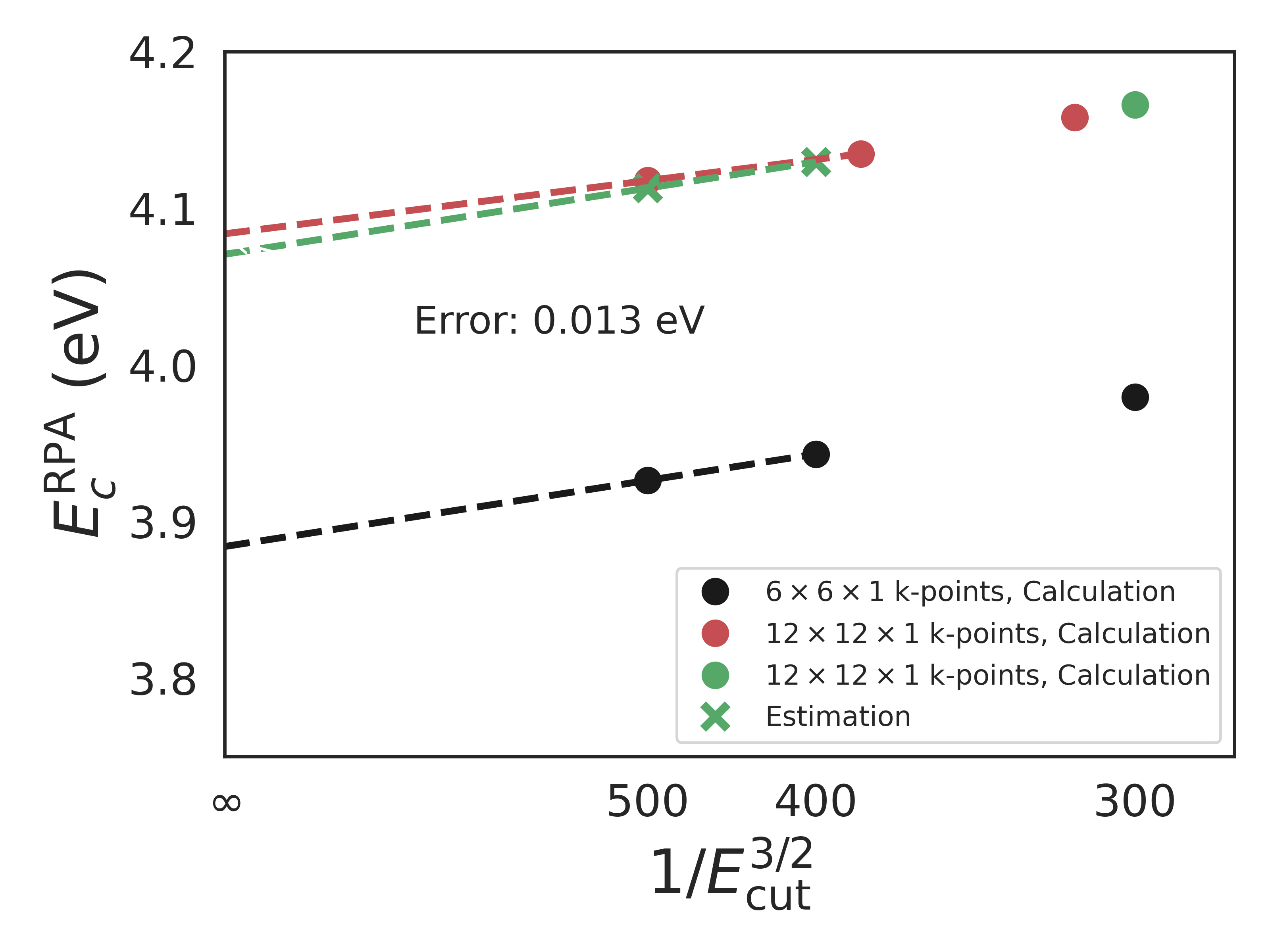
The RPA calculations were carefully converged with respect to plane wave basis using the following extrapolation scheme: In the following figure, the black dots are from a calculation with \(6\times6\times1\) k-points (not enough to achieve convergence) but high cutoff energies (300, 400, 500 eV). The green circle is a calculation at a much denser k-point sampling of \(12\times12\times1\) (converged). From these four circles, the two green crosses are predicted which allow for an extrapolation to infinite cutoff energy. The red dots represent actual calculations with both a dense k-point grid and high cutoff energies to test the extrapolation scheme. The error introduced by the extrapolation scheme for this particular system is seen to be 0.013 eV. The k-point grid of \(12\times12\times1\) ensures that the exchange + correlation energy is converged to within 0.02 eV with respect to the k-point density.