Perovskite water-splitting¶

We perform computational screening of around 19 000 oxides, oxynitrides, oxysulfides, oxyfluorides, and oxyfluoronitrides in the cubic perovskite structure with photoelectrochemical cell applications in mind.

Castelli, I. E., Landis, D. D., Thygesen, K. S., Dahl, S., Chorkendorff, I., Jaramillo, T. F., and Jacobsen, K. W.

New cubic perovskites for one- and two-photon water splitting using the computational materials repository.

Energy Environ. Sci. 5, 9034.

Castelli, I. E., Olsen, T., Datta, S., Landis, D. D., Dahl, S., Thygesen, K. S., and Jacobsen, K. W.

Computational screening of perovskite metal oxides for optimal solar light capture.

Energy Environ. Sci. 5, 5814.

Castelli, I. E., Thygesen, K. S., and Jacobsen, K. W.

Calculated Pourbaix Diagrams of Cubic Perovskites for Water Splitting: Stability Against Corrosion.

Topics in Catalysis 57, 265.

Key-value pairs¶

key	description	unit
A_ion	A-ion in the cubic perovskite
B_ion	B-ion in the cubic perovskite
CB_dir	Direct position of the conduction band edge
CB_ind	Indirect position of the conduction band edge
VB_dir	Direct position of the valence band edge
VB_ind	Indirect position of the valence band edge
anion	Anion combination in the perovskite
combination	General formula
gllbsc_dir_gap	Direct bandgap calculated with GLLB-SC	eV
gllbsc_ind_gap	Indirect bandgap calculated with GLLB-SC	eV
heat_of_formation_all	Heat of formation calculated with respect to all the materials in the pool of references	eV
project	project
reference	standard (used to calculate the standard heat of formation) or pool (reference included in the calculation of the convex hull)
standard_energy	standard_energy

ABO3 candidates for water splitting¶

from __future__ import print_function
import ase.db
from ase.phasediagram import PhaseDiagram

con = ase.db.connect('cubic_perovskites.db')

references = [(row.formula, row.energy)
              for row in con.select('reference')]

with open('abo3.csv', 'w') as fd:
    print('# id, formula, heat of formation [eV/atom]', file=fd)
    for row in con.select(combination='ABO3'):
        pd = PhaseDiagram(references, filter=row.formula, verbose=False)
        energy = pd.decompose(row.formula)[0]
        heat = (row.energy - energy) / row.natoms
        if (heat < 0.21 and
            (3.1 > row.gllbsc_ind_gap > 1.4 or
             3.1 > row.gllbsc_dir_gap > 1.4) and
            (row.VB_ind - 4.5 > 1.23 and row.CB_ind - 4.5 < 0 or
             row.VB_dir - 4.5 > 1.23 and row.CB_dir - 4.5 < 0)):
            formula = row.A_ion + row.B_ion + row.anion
            print('{0}, {1}, {2:.3f}'.format(row.id, formula, heat), file=fd)

The 10 candidates are:

# id	formula	heat of formation [eV/atom]
14300	SrSnO3	0.020
14363	CaSnO3	0.164
14410	LiVO3	0.171
14425	CsNbO3	0.176
14688	BaSnO3	-0.084
14863	AgNbO3	0.207
14981	SnTiO3	0.103
15088	NaSbO3	0.205
15292	SrGeO3	0.157
15621	CaGeO3	0.158

Here are the band gaps:

import matplotlib.pyplot as plt
import ase.db
con = ase.db.connect('cubic_perovskites.db')

rows = []
for i, line in enumerate(open('abo3.csv')):
    if line[0] == '#':
        continue
    id, formula = line.split(',')[:2]
    id = int(id)
    row = con.get(id)
    rows.append(row)
    plt.text(i - 1.25, -1.9, formula, rotation=60)

N = len(rows)
assert N == 10
x = range(N)
y = [(row.VB_ind + row.CB_ind) / 2 - 4.5 for row in rows]
dyd = [row.gllbsc_dir_gap / 2 for row in rows]
dyi = [row.gllbsc_ind_gap / 2 for row in rows]
plt.errorbar(x, y, dyd, color='k', lw=0, mew=2, elinewidth=2,
             label='Direct Gap')
plt.errorbar(x, y, dyi, color='r', lw=0, mew=2, elinewidth=2,
             label='Indirect Gap')
plt.xlim(-1, N)
plt.ylim(4.4, -2.2)
plt.axhline(y=0, xmin=-1, xmax=N, lw=2, color='b', ls='dashed')
plt.axhline(y=1.23, xmin=-1, xmax=N, lw=2, color='g', ls='dotted')
plt.text(N + 0.1, 0.2, 'H$^+$/H$_2$', color='b')
plt.text(N + 0.1, 1.43, 'O$_2$/H$_2$O', color='g')
plt.ylabel('Potential (V vs NHE) [eV]')
plt.xticks([-1], '')
plt.legend(loc=4)
plt.savefig('abo3.svg')

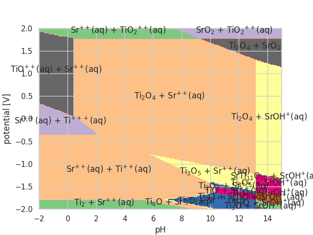
The stability of a material with respect to solid and dissolved phases can be evaluated using Pourbaix diagrams. Here how to generate the Pourbaix diagram for SrTiO3:

# creates: SrTiO3_pourbaix.png
import numpy as np
import matplotlib.pyplot as plt
import ase.db
from ase.phasediagram import Pourbaix, solvated

con = ase.db.connect('cubic_perovskites.db')

refs = []
for row in con.select('reference'):
    refs.append((row.formula, row.standard_energy))

# Add other solid/dissolved phases not included before:
refs += [('Ti6O', -5.443), ('Ti2O3', -13.907), ('Ti2O', -5.164),
         ('TiO', -4.838), ('SrO2', -5.356), ('Ti3O', -5.346),
         ('Ti3O5', -22.917), ('Sr4Ti3O10', -50.756), ('SrTi11O20', -93.313)]

# Extract the dissolved phases:
refs += solvated('SrTi')

pb = Pourbaix(refs, formula='SrTiO3')
U = np.linspace(-2, 2, 200)
pH = np.linspace(-2, 15, 300)
d, names, text = pb.diagram(U, pH, plot=True, show=False)

plt.savefig('SrTiO3_pourbaix.png')

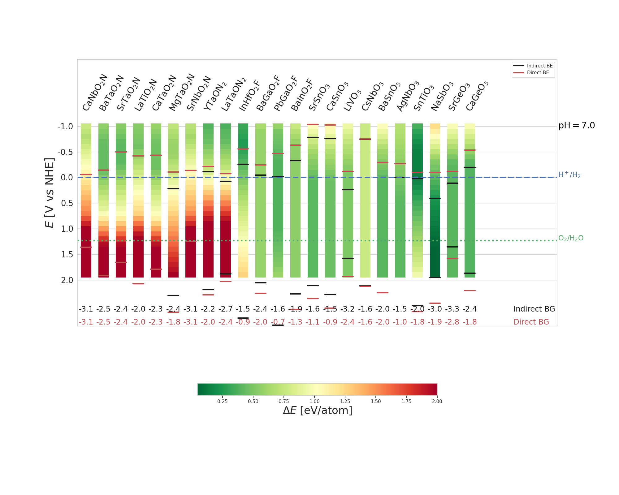
Here how to plot the energy differences for all (oxides: 10, oxynitrides: 7, oxyfluorides: 3) the candidate material and the most stable experimental known solid and dissolved phases at pH = 7 and for a potential between -1 and 2 V:

# creates: WS_pourbaix.png
import numpy as np
import matplotlib.pyplot as plt
import matplotlib.cm as cm
from matplotlib.collections import PatchCollection
import matplotlib.patches as patches
import ase.db
from ase.phasediagram import Pourbaix, solvated

con = ase.db.connect('cubic_perovskites.db')

pH = 7.
Us = np.arange(-1, 2, 0.1)
E0 = -4.5
lb = -0.5  # lower bound for the energy scale
ub = 2.0  # upper bound for the energy scale

info = []
xs = []
ys = []
heats = []

for row in con.select('heat_of_formation_all<=0.21'):
    if (row.gllbsc_ind_gap >= 1.4 and row.gllbsc_ind_gap <= 3.1 and
        row.CB_ind <= 0 - E0 and row.VB_ind >= 1.23 - E0) or \
       (row.gllbsc_dir_gap >= 1.4 and row.gllbsc_dir_gap <= 3.1 and
        row.CB_dir <= 0 - E0 and row.VB_dir >= 1.23 - E0):
        name = row.A_ion + row.B_ion + row.anion
        energy = row.standard_energy

        info.append([name, row.gllbsc_ind_gap + E0, row.gllbsc_dir_gap + E0,
                     row.VB_ind + E0, row.CB_ind + E0,
                     row.VB_dir + E0, row.CB_dir + E0])

        refs = []
        for row_ref in con.select('reference'):
            refs.append((row_ref.formula, row_ref.standard_energy))

        # Extract the dissolved phases:
        refs += solvated(row.A_ion + row.B_ion)

        for U in Us:
            pb = Pourbaix(refs, name)
            results, refs_energy = pb.decompose(U, pH, verbose=False)
            Ediff = (energy - refs_energy) / 5
            Ediff = min(Ediff, ub)
            Ediff = max(Ediff, lb)
            xs.append(len(info) - 1)
            ys.append(U)
            heats.append(Ediff)

fig = plt.figure(figsize=(20, 16))
ax = fig.add_subplot(111)

cx = 0.3
cy = 0.05
rects = []
for i in range(len(heats)):
    rect = patches.Rectangle((xs[i] - cx, ys[i] - cy), 2 * cx, 2 * cy)
    rects.append(rect)
p = PatchCollection(rects, edgecolors=None, linewidths=0, cmap=cm.RdYlGn_r)
p.set_array(np.array(heats))
ax.add_collection(p)

for i in range(len(info)):
    plt.plot([i - cx, i + cx], [info[i][3], info[i][3]], '-',
             color='k', linewidth=3)
    plt.plot([i - cx, i + cx], [info[i][4], info[i][4]], '-',
             color='k', linewidth=3)
    plt.plot([i - cx, i + cx], [info[i][5], info[i][5]], '-',
             color='r', linewidth=3)
    plt.plot([i - cx, i + cx], [info[i][6], info[i][6]], '-',
             color='r', linewidth=3)
    plt.text(i, 2.5, round(info[i][1], 1), color='k', fontsize=17.5,
             verticalalignment='top', horizontalalignment='center')
    plt.text(i, 2.75, round(info[i][2], 1), color='r', fontsize=17.5,
             verticalalignment='top', horizontalalignment='center')
plt.plot([cx, cx], [info[0][3], info[0][3]], '-', color='k', linewidth=3,
         label='Indirect BE')
plt.plot([cx, cx], [info[0][5], info[0][5]], '-', color='r', linewidth=3,
         label='Direct BE')
plt.text(len(info) + 1.5, 2.5, 'Indirect BG', color='k', fontsize=17.5,
         verticalalignment='top', horizontalalignment='left')
plt.text(len(info) + 1.5, 2.75, 'Direct BG', color='r', fontsize=17.5,
         verticalalignment='top', horizontalalignment='left')

for i in range(len(info)):
    formula = info[i][0]
    for j in range(10):
        if str(j) in formula:
            formula = formula.replace(str(j), "$_" + str(j) + "$")
    plt.text(i - cx, -1.25, formula, rotation=60, va='bottom', ha='left',
             fontsize=20.5, color='k')

xmax = len(info) + 4
plt.text(xmax + 0.05, -1, 'pH$=' + str(pH) + '$', color='black', fontsize=20.5,
         verticalalignment='center')
plt.axhline(1.23, xmin=0, xmax=xmax, color='g', ls='dotted', lw=3.5)
plt.text(xmax + 0.05, 1.23, 'O$_2$/H$_2$O', color='g', fontsize=16.5)
plt.axhline(0, xmin=0, xmax=xmax, color='b', ls='dashed', lw=3.5)
plt.text(xmax + 0.05, 0, 'H$^+$/H$_2$', color='b', fontsize=16.5)

cbar = plt.colorbar(p, orientation='horizontal', shrink=0.5)
cbar.set_label(r'$\Delta E$ [eV/atom]', fontsize=24.5)

plt.ylabel('$E$ [V vs NHE]', fontsize=26.5)
plt.yticks([-1, -0.5, 0, 0.5, 1, 1.5, 2],
           ['-1.0', '-0.5', '0.0', '0.5', '1.0', '1.5', '2.0'],
           fontsize=18.5)
plt.xticks([])
plt.legend()
plt.xlim(xmin=-0.5, xmax=xmax)
plt.ylim(ymin=-2.3, ymax=2.9)
plt.gca().invert_yaxis()

plt.savefig('WS_pourbaix.png')

Perovskite water-splitting¶

Key-value pairs¶

ABO3 candidates for water splitting¶

Table of Contents

Previous topic

Next topic

This Page