Database of ABX2 materials

Database contains chalcopyrite, kesterite, and wurtzite polymorphs of II–IV–V2 and III–III–V2 materials investigated for light absorption in the visible range. The data set includes stability information, band gaps, and carrier effective masses.

Mohnish Pandey, Korina Kuhar, and Karsten W. Jacobsen

II–IV–V2 and III–III–V2 Polytypes as Light Absorbers for Single Junction and Tandem Photovoltaic Devices

10. Phys. Chem. C, 2017, 121 (33), pp 17780–17786

The data

• Download database: abx2.db

• Browse data

Key-value pairs

key	description	unit
E_hull	E-hull	eV
KS_gap	Kohn Sham band gap	eV
m_e	Effective electron mass	\(m_e\)
m_h	Effective hole mass	\(m_e\)
Dxc	Derivative discontinuity (GLLB-SC)	eV
E_relative_perAtom	Energy per atom	eV
E_uncertanty_hull	Uncertanty of the convex hull energy	eV
E_uncertanty_perAtom	Uncertanty of the total energy	eV
GLLB_dir	Direct band gap (GLLB-SC)	eV
GLLB_ind	Indirect band gap (GLLB-SC)	eV
TB09_dir	Direct band gap (TB09)	eV
TB09_ind	Indirect band gap (TB09)	eV
lattice	Crystal system
phase	Phase
short_name	Short chemical formula
total_en	Total energy (mBEEF)	eV

Example

mBEEF energies and the corresponding uncertainties for three phases:

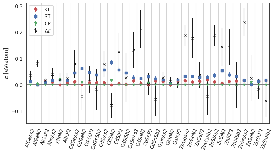
# creates: enthalpy.png
import numpy as np
import matplotlib.pyplot as plt
from ase.db import connect

db = connect('abx2.db')
names = sorted(row.short_name for row in db.select(phase='ST'))
x = np.arange(len(names))

plt.figure(figsize=(10, 5))

for phase, mark, color in zip(['KT', 'ST', 'CP'], 'osv', 'rbg'):
    y = []
    dy = []
    for row in db.select(phase=phase, sort='short_name'):
        y.append(row.E_relative_perAtom)
        dy.append(row.E_uncertanty_perAtom)
    print(x, y)
    plt.errorbar(x, y, yerr=dy, color=color, fmt=mark, label=phase)

y = []
dy = []
for row in db.select(phase='ST', sort='short_name'):
    y.append(row.E_hull)
    dy.append(row.E_uncertanty_hull)
plt.errorbar(x, y, yerr=dy, color='k', fmt='x', label=r'$\Delta E$')
plt.xticks(x, names, rotation=70)
for xx in x:
    plt.axvline(xx + 0.5, color='lightgrey')
plt.axhline(0, color='grey')
plt.xlim(-0.5, x[-1] + 0.5)
plt.legend()
plt.ylabel(r'$E$ [eV/atom]')
plt.savefig('enthalpy.png', bbox_inches='tight')