Rasmussen, F., Thygesen, K. S.
Phys. Chem. C, 2015, 119 (23), pp 13169–13183, April 30, 2015
This database contains calculated structural and electronic properties of a range of 2D materials. The database contains the results presented in the following paper:
Rasmussen, F., Thygesen, K. S.
Phys. Chem. C, 2015, 119 (23), pp 13169–13183, April 30, 2015
Download raw data: c2dm.db
The structures were first relaxed using the PBE xc-functional and a 18x18x1 k-point sampling until all forces on the atoms where below 0.01 eV/Å. The rows with xc=’PBE’ contains data from these calculations.
For materials that were found to be semiconducting in the PBE calculations we furthermore performed calculations using the LDA and GLLB-SC xc functionals and the lattice constants and atom positions found from the PBE calculation. For these calculations we used a 30x30x1 k-point sampling. For the GLLB-SC calculations we calculated the derivative discontinuity and have added this contribution to the electronic band gaps. Data for these calculations are found in rows with xc=’GLLBSC’ and xc=’LDA’, respectively.
Furthermore, we calculated the G0W0 quasiparticle energies using the wavefunctions and eigenvalues from the LDA calculations and a plane-wave cut-off energy of at least 150 eV. The quasiparticle energies where further extrapolated to infinite cut-off energy via the methods described in the paper. The LDA rows thus further have key-value pairs with the results from the G0W0 calculations.
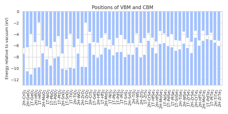
The following python script shows how to plot the positions of the VBM and CBM.
# creates: band-alignment.png
from math import floor, ceil
import re
import numpy as np
import matplotlib.pyplot as plt
import ase.db

# Connect to database
db = ase.db.connect('c2dm.db')

# Select the rows that have G0W0 results
rows = db.select('xc=LDA,ind_gap_g0w0>0')

data = []
for row in rows:
    name = row.name
    # Use regular expressions to get the atomic species from the name
    m = re.search('([A-Z][a-z]?)([A-Z][a-z]?)2', name)
    M = m.group(1)
    X = m.group(2)

    label = ''
    if row.phase == 'H':
        label += '2H-'
    elif row.phase == 'T':
        label += '1T-'
    label += name.replace('2', '$_2$')

    # Store data as tuples - easier to sort
    data.append((M, X, label, row.vbm_g0w0, row.cbm_g0w0))

# Sort according to atomic species (alphabetically)
data.sort(key=lambda tup: (tup[1], tup[0]))
label_list = [tup[2] for tup in data]
vbm_list = [tup[3] for tup in data]
cbm_list = [tup[4] for tup in data]

x = np.arange(len(vbm_list))
emin = floor(min(vbm_list)) - 1.0
emax = ceil(max(cbm_list)) + 1.0

# With and height in pixels
ppi = 100
figw = 800
figh = 400

fig = plt.figure(figsize=(figw / ppi, figh / ppi), dpi=ppi)
ax = fig.add_subplot(1, 1, 1)
ax.bar(x + 0.1, np.array(vbm_list) - emin, bottom=emin, color='#A3C2FF')
ax.bar(x + 0.1, emax - np.array(cbm_list), bottom=cbm_list, color='#A3C2FF')
ax.set_xlim(0, len(vbm_list))
ax.set_ylim(emin, emax)
ax.set_xticks(x + 0.5)
ax.set_xticklabels(label_list, rotation=90, fontsize=10)
ax.tick_params(axis='y', labelsize=10)

plt.title('Positions of VBM and CBM', fontsize=12)
plt.ylabel('Energy relative to vacuum (eV)', fontsize=10)
plt.tight_layout()
plt.savefig('band-alignment.png')
This produces the figure