Quantum Point Defects in 2D Materials (QPOD) Database

If you are using data from this database in your research, please cite the following papers:

Bertoldo, F., Ali, S., Manti, S., Thygesen, K. S.

Quantum point defects in 2D materials - the QPOD database

npj Comput Mater 8, 56 (2022)

• Browse data: The webpage is temporarily down due to maintenance

• Download database: The database is temporarily unavailable due to maintenance

Brief description

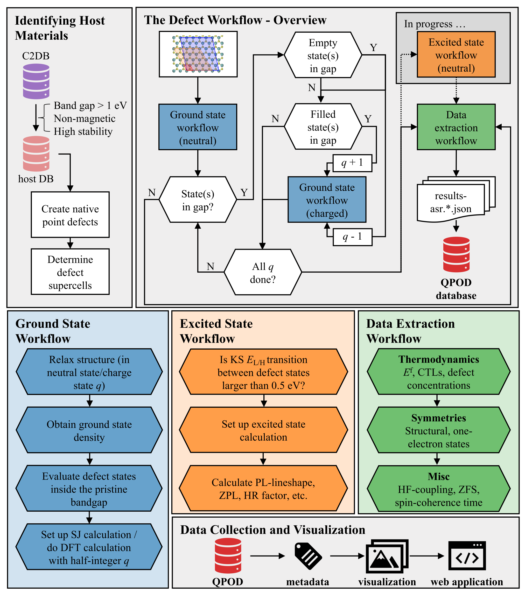
The database contains structural, thermodynamic, electronic, magneto-optical, of 500 distinct intrinsic point defects in 2D Materials. The properties are calculated by density functional theory (DFT) as implemented in the GPAW electronic structure code. The workflow was constructed using the Atomic Simulation Recipes (ASR) and executed with the MyQueue task manager. For each defect, different charge states are available resulting in more than 2000 rows for this database.

Overview of methods and parameters used

If a parameter is not specified at a given step, its value equals that of the last step where it was specified:

Workflow step(s)	Parameters
Structure and energetics(*)	\(k\)-point density = 6.0/Å\(^{-1}\); Fermi smearing = 0.02 eV; PW cutoff = 800 eV; xc functional = PBE; maximum force = 0.01 eV/Å;
PBE electronic properties (*)	\(k\)-point density = \(12.0/\mathrm{Å}^{-1}\)

(*) For the cases with convergence issues, we increased the smearing to 0.05, 0.08, 0.1 eV.

Funding acknowledgements

The QPOD project has received funding from the Danish National Research Foundation’s Center for Nanostructured Graphene (CNG) and the European Research Council (ERC) under the European Union’s Horizon 2020 research and innovation program Grant No. 773122 (LIMA) and Grant agreement No. 951786 (NOMAD CoE).

Versions

Version	rows	comment
2022-03-31	2061	Initial release
2022-06-09	2061	Added spin coherence times for 69 triplet centers in 45 different host materials (see related manuscript here)
2022-07-11	2061	Web panel update for improved readability

Examples

Ionization potentials (IPs) and electron affinities (EAs)

The following Python script shows how to plot IPs and EAs with and without relaxation effects included for systems within a given list of hosts (similar to Fig. 12 from the QPOD paper).

# creates: fig12.png
from ase.db import connect
from ase.formula import Formula
import matplotlib.pyplot as plt
import numpy as np
from math import floor


def get_plot_data(db, hosts):
    """Return data needed for subsequent plotting."""
    # list of tuples of relaxed EA, IP (one tuple for each defect)
    relaxed = []

    # list of tuples of unrelaxed EA, IP (one tuple for each defect)
    unrelaxed = []

    names = []  # list of corresponding defect system names
    vbms = []  # list of pristine VBMs
    cbms = []  # list of pristine CBMs

    # Extract all entries of QPOD, where CTLs have been calculated, i.e.
    # 'has_asr_sj_analyze=True' (CTLs calculated from SJ theory).
    # The full amount of data is always stored in the '(charge 0)'
    # charge state of a particular defect.
    for i, row in enumerate(db.select(has_asr_sj_analyze=True,
                                      charge_state='(charge 0)')):
        # only show systems from the given list of hosts for this plot
        if row.host_name in hosts:
            # get the results from asr.sj_analyze
            # (recipe to calculate formation energies and CTLs)
            sjres = row.data['results-asr.sj_analyze.json']
            # the particular CTLs are stored in the 'transitions'
            # keyword of the results
            transitions = sjres['kwargs']['data']['transitions']
            # get pristine results to know where the band edges are
            pristine = sjres['kwargs']['data']['pristine']['kwargs']['data']
            vbm = pristine['vbm']
            cbm = pristine['cbm']
            # each row has a row.defect name where the name of the
            # defect is stored the next six lines are simiply here
            # to format it nicely
            defecttype = row.defect_name.split('_')[0]
            defectkind = row.defect_name.split('_')[1]
            if defecttype == 'v':
                defecttype = 'V'
            host = Formula(row.host_name)
            host = f'{host:latex}'
            # loop over all CTLs for the current defect system
            for trans in transitions:
                transr = trans['kwargs']['data']
                name = transr['transition_name']
                # CTL 0/1 corresponds to the EA
                if name == '0/1':
                    val = transr['transition_values']['kwargs']['data']
                    ea = val['transition'] + val['erelax'] - val['evac']
                    ea_un = val['transition'] - val['evac']
                # CTL 0/-1 corresponds to the EA
                elif name == '0/-1':
                    val = transr['transition_values']['kwargs']['data']
                    ip = val['transition'] - val['erelax'] - val['evac']
                    ip_un = val['transition'] - val['evac']
            # append the newly extracted EA, IP, VBM, CBM to the
            # respective lists
            vbms.append(vbm)
            cbms.append(cbm)
            relaxed.append((ea, ip))
            unrelaxed.append((ea_un, ip_un))
            names.append(
                rf"{defecttype}$_\mathrm{'{'}{defectkind}{'}'}$ in {host}")

    return relaxed, unrelaxed, vbms, cbms, names


def plot(filename):
    # connect to the QPOD database
    db = connect('qpod.db')

    # extract plotting data for a given subset of host materials
    # relaxed EA/IP, unrelaxed EA/IP, VBMs, CBMs, names of defect systems
    hosts = ['BN', 'SnTe', 'K2I2', 'ZnI2', 'PbCl2', 'Al2Cl6']
    relaxed, unrelaxed, vbms, cbms, names = get_plot_data(db, hosts)

    # the actual plotting is happening here:
    # matplotlib setup
    fig, ax = plt.subplots(figsize=(8, 4.8))
    # plot the IPs, EAs for all extracted defect systems
    plot_transitions(ax, relaxed, unrelaxed, vbms, cbms, names)
    plt.tight_layout()
    plt.savefig(filename)
    # plt.show()


def plot_transitions(ax, relaxed, unrelaxed, vbms, cbms, names):
    # define x-axis, find lowest lying VBM
    x = np.arange(len(vbms)) - 0.5
    emin = floor(min(vbms)) - 1.0

    # loop over all values for rel., unrel. IP/EA and plot them
    for i in range(len(relaxed)):
        ax.scatter([i - 0.5], [relaxed[i][0]],
                   marker='s', edgecolors='C3', facecolors='none')
        ax.scatter([i - 0.5], [unrelaxed[i][0]],
                   marker='x', color='C3')
        ax.scatter([i - 0.5], [relaxed[i][1]],
                   marker='s', edgecolors='C0', facecolors='none')
        ax.scatter([i - 0.5], [unrelaxed[i][1]],
                   marker='x', color='C0')

    # plot pristine band edges
    ax.bar(x, np.array(vbms) - emin, bottom=emin, color='grey', alpha=0.5)
    ax.bar(x, -np.array(cbms) + 2, bottom=cbms, color='grey', alpha=0.5)

    # define legends for IP/EA with/without relaxation included
    ax.scatter([], [], marker='s', facecolors='none', edgecolors='C3',
               label='-IP w/ relax: (0/+1)')
    ax.scatter([], [], marker='s', facecolors='none', edgecolors='C0',
               label='EA w/ relax: (0/-1)')
    ax.scatter([], [], marker='x', color='C3', label='-IP w/o relax: (0/+1)')
    ax.scatter([], [], marker='x', color='C0', label='EA w/o relax: (0/-1)')

    # set limits, labels, and ticks for the plot
    ax.set_ylabel(r'$E-E_{\mathrm{vac}}$ [eV]')
    ax.set_ylim(emin, 1.5)
    ax.set_xlim(-1, len(relaxed) - 1)
    ax.set_ylabel(r'$E-E_{\mathrm{vac}}$ [eV]')
    ax.set_xlim(-1, len(relaxed) - 1)
    ax.set_xticks(x)
    ax.set_xticklabels(names, rotation=90)
    ax.legend(loc='lower left')


plot('fig12.png')

This produces the figure

Tools for creating the “QPOD” database

Requirements

Python 3.7+ and up-to-date versions of ASE, ASR and GPAW.

Workflow

The workflow was executed using MyQueue. The corresponding workflow script will follow shortly.