Impurities in 2D Materials Database

If you are using data from this database in your research, please cite the following paper:

Absorption versus Adsorption: High-Throughput Computation of Impurities in 2D Materials

Joel Davidsson, Fabian Bertoldo, Kristian S. Thygesen, Rickard Armiento

arXiv:2207.05353 (cond-mat)

Please also cite the related DOI for the actual data:

Interstitial and Adsorbate Structure Database

Joel Davidsson, Fabian Bertoldo, Kristian S. Thygesen, Rickard Armiento

DOI 10.11583/DTU.19692238

• Browse data

• Download database: imp2d.db

Brief description

This database contains structural, thermodynamic, and electronic data of more than 17,500 single impurity defects over a set of 53 experimentally synthesized 2D monolayers. The defect structures (interstitials, adsorption sites) were set up with the ASE DefectBuilder module. The computational workflow was implemented with the httk High-Throughput Toolkit. 12,813 of the overall 17,364 systems have reached full ionic convergence as described in the publication above.

Overview of methods and parameters used

If a parameter is not specified at a given step, its value equals that of the last step where it was specified:

Workflow step(s)	Parameters
Initial relaxation	Electronic structure code: VASP; xc functional = PBE; \(k\)-point grid: Gamma-point only; spin-polarized; PW energy cutoff = 600 eV; kinetic energy cutoff = 900 eV; electronic tolerance (energy) = 10`^{-4}`; ionic tolerance (energy) = 0.005 eV; FFT grid = 3/2
Final relaxation	Electronic structure code: VASP; xc functional = PBE; \(k\)-point grid: Gamma-point only; spin-polarized; PW energy cutoff = 600 eV; kinetic energy cutoff = 900 eV; electronic tolerance (energy) = 10`^{-6}`; ionic tolerance (energy) = 0.0001 eV; FFT grid = 2

Funding acknowledgements

The project has received funding from the Danish National Research Foundation’s Center for Nanostructured Graphene (CNG) and the European Research Council (ERC) under the European Union’s Horizon 2020 research and innovation program Grant No. 773122 (LIMA) and Grant agreement No. 951786 (NOMAD CoE). We acknowlege funding from the Swedish eScience Centre (SeRC) and support from the Swedish REsearch Council (VR) Grant No. 2020-05402. The computations were enabled by resources provided by the Swedish National Infrastructure for Computing (SNIC) at NSC and PDC partially funded by the Swedish Research Council through Grant Agreement No. 2018-05973.

Versions

Version	rows	comment
2022-07-12	17364	Initial release

Key-value pairs

key	description	unit
host	Host chemical formula
dopant	Impurity species
defecttype	Impurity type
eform	Formation energy	eV
site	Defect setup position
depth	Depth parameter
extension_factor	Extension factor
en2	Total energy	eV
conv2	Total energy convergence	eV
spin	Magnetic moment
supercell	Calculation supercell
host_spacegroup	Host spacegroup symbol
converged	Relaxation converged?
name	System name
en1	Total energy, first WF step	eV
conv1	Total energy convergence, first WF step	eV
dopant_chemical_potential	Dopant chemical potential	eV
hostenergy	Host energy	eV

Examples

Formation energies for period 4 transition metal impurities in MoSe2

The following Python script shows how to plot the formation energies of period 4 transition metal impurities (for different interstitial and adsorption sites).

# creates: formation_energies_MoSe2.png
from ase.data import atomic_numbers
from ase.db import connect
import matplotlib.pyplot as plt


def get_plot_data(db, hosts, dopants):
    """Return data needed for subsequent plotting."""
    eforms = []
    numbers = []
    defecttypes = []
    # loop over all given host materials
    for host in hosts:
        # loop over all given dopants
        for dopant in dopants:
            # only include data that is fully converged and relaxed
            for row in db.select(host=host, dopant=dopant, converged=True):
                # convert dopant string to atomic number and append to list
                numbers.append(atomic_numbers[dopant])
                # extract formation energy and defecttype
                # (interstitial or adsorbate)
                eforms.append(row.eform)
                defecttypes.append(row.defecttype)

    return eforms, numbers, defecttypes


def plot(filename):
    # connect to the 'Impurities in 2D Materials database'
    db = connect('imp2d.db')

    # extract plotting data for group 4 transition metal doped MoSe2
    hosts = ['MoSe2']
    dopants = ['Sc', 'Ti', 'V', 'Cr', 'Mn', 'Fe', 'Co', 'Ni', 'Cu', 'Zn']
    eforms, numbers, defecttypes = get_plot_data(db, hosts, dopants)

    # the actual plotting is happening here:
    # matplotlib setup
    fig, ax = plt.subplots(figsize=(6, 3.8))
    # plot the formation energies for the period 4 TM-impurities in MoS2
    for i in range(len(eforms)):
        if defecttypes[i] == 'interstitial':
            color = 'C0'
        elif defecttypes[i] == 'adsorbate':
            color = 'C1'
        # plot formation energy versus dopant element
        ax.scatter(numbers[i], eforms[i], marker='.', color=color)
    # set title
    ax.set_title(r'MoSe$_2$ impurities')
    # set up the legend
    ax.scatter([], [], marker='.', color='C0',
               label='interstitial')
    ax.scatter([], [], marker='.', color='C1',
               label='adsorbate')
    ax.legend()
    # fix xticks
    ax.set_xticks(list(set(numbers)))
    ax.set_xticklabels(dopants)
    # set x- and y-label
    ax.set_xlabel(r'Dopant element')
    ax.set_ylabel(r'Formation energy [eV]')
    # set plot limits
    ax.set_ylim(0, 5)
    # save figure
    plt.tight_layout()
    plt.savefig(filename)
    # plt.show()


plot('formation_energies_MoSe2.png')

This produces the figure

Tools for creating the database

Software used

VASP, httk, Python, and ASE.

Defect setup

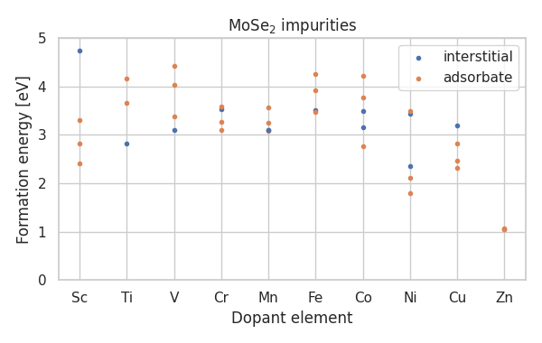
The defect setup was inspired by the work of J. Davidsson for ADAQ and generalized in the ASE DefectBuilder. Find more information, explanations, and some code examples in the documentation of the DefectBuilder.

Workflow

The workflow was executed using httk.